Linear regression is a foundational technique in machine learning and statistics, serving as a cornerstone for more complex algorithms. In this blog post, we’ll dive deep into linear regression, exploring its concepts, applications, and implementation using Python. Whether you’re a beginner or looking to refresh your knowledge, this guide will equip you with the tools to understand and apply linear regression effectively.

Table of Content

Introduction

What is Linear Regression?

Fundamentally, linear regression is a statistical technique for simulating the relationship between one or more independent variables and a dependent variable. The goal is to find a linear equation that best fits the data, allowing us to make predictions or understand the impact of variables on the outcome.

The Evolution of Regression Analysis: A Historical Journey

The concept of regression has a rich history spanning over two centuries:

1. The Foundation (1800s) Francis Galton pioneered regression analysis while studying heredity. His groundbreaking research on parent-child height relationships revealed a crucial statistical phenomenon: extremely tall parents typically had children closer to average height, introducing the concept of “regression toward the mean.”
2. Statistical Revolution (Early 1900s) Two statistical giants shaped regression’s theoretical foundation:

• Karl Pearson formalized correlation coefficients and parameter estimation
• Ronald Fisher revolutionized the field by developing analysis of variance (ANOVA) and introducing maximum likelihood estimation

3. Computational Era (1950s-1970s) The advent of computers transformed regression analysis:

• Large-scale data processing became possible
• Complex statistical calculations could be performed rapidly
• Multiple regression analysis became practical for researchers

4. Methodological Expansion (1980s-1990s) Regression techniques diversified significantly:

• Stepwise regression emerged for variable selection
• Logistic regression gained prominence in categorical data analysis
• New diagnostic tools improved model validation

5. Modern Applications (2000s-Present) Regression continues to evolve:

• Serves as a foundation for machine learning algorithms
• Powers predictive analytics and forecasting
• Integrates with advanced statistical methods
• Supports big data analysis and artificial intelligence applications

This brief history showcases regression’s journey from a simple heredity study tool to a cornerstone of modern statistical analysis and predictive modeling.

Goal of Linear Regression:

The goal is to find the best line that fits all data points in a straight line that explains the relationship with minimum errors.

The simplest form of linear regression, known as simple linear regression, involves only one independent variable and can be represented by the equation:

y = mx + b

Where:

• y is the dependent variable (what we’re trying to predict)
• x is the independent variable
• m denotes the slope of the line, or how much y changes for every unit change in x
• b is the y-intercept (the value of y when x is 0)

When dealing with multiple independent variables, we use multiple linear regression, which extends this concept to higher dimensions.

Linear Algebra: Slope and Intercept Concept

Slope (m)

The rate of change of the dependent variable with respect to the independent variable in a linear relationship. Shows the “tilt” of the line.

• It represents a line’s steepness or rate of change
• Calculated as the change in y divided by change in x (rise over run)
• Formula: m = (y2 – y1)/(x2 – x1)
• It indicates the amount that y varies for every unit change in x

Example: If sales increase by $500 for every $1000 spent on advertising:

• Slope = 500/1000 = 0.5
• This means for every $1 spent on advertising, sales increase by $0.50

Intercept (b)

The value of the dependent variable when the independent variable is zero in a linear relationship. Shows the “Shift” of the line

• It is the point where the line crosses the y-axis when x = 0
• Represents the base value of y when x equals zero
• In equation y = mx + b, b is the y-intercept

Example: In a sales model where:

• Base sales (without advertising) = $10,000 (y-intercept)
• Sales = 0.5x + 10000
  • If advertising (x) = $0, sales = $10,000
  • If advertising = $1000, sales = 0.5(1000) + 10000 = $10,500

Types of Linear Regression

Simple Linear Regression

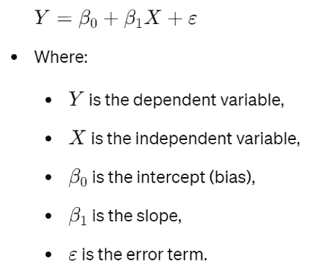
Simple linear regression models the relationship between one independent variable (X) and one dependent variable (Y) using a straight-line equation.

General Form

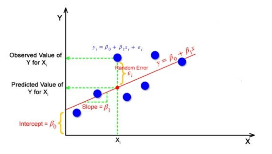
Example: Predicting House Price by House Area only

Multiple Linear Regression

Multiple linear regression models the relationship between multiple independent variables (𝑋1,𝑋2,.. ,Xn​) and one dependent variable (Y) using a linear equation.

General Form

Example: Predicting house price by house area, number of bedrooms and bathrooms, age of house, population of near by area, distance between nearest hospital, school, etc.

Algorithm: How do we find the best fit line?

The goal is to find the perfect line that best fits our data by optimizing two key parameters: slope and intercept. This line should minimize the gap between what our model predicts and what we actually observe in our data.

Linear Regression can be model data in two different ways

Ordinary Least Squares (OLS)

OLS is an analytical method that directly computes the optimal parameters by minimizing the sum of squared differences between observed and predicted values.

• A method to find the best-fitting line by minimizing the sum of squared differences between predicted and actual values
• It is a deterministic algorithm. Thus, if run multiple times, it will always converge to the same weights
• Direct calculation approach using a mathematical formula
• Best for smaller datasets with exact solutions
• It always finds the optimal solution
• It has no hyperparameters

Key Characteristics:

1. Formula: β = (X’X)^(-1)X’y
   • β: coefficients
   • X: input variables, X’ is transpose of X
   • y: target variable
2. Advantages:
   • Provides exact solution
   • Fast for small datasets
   • No iterations needed
   • Guaranteed optimal solution
3. Limitations:
   • Computationally expensive for large datasets
   • Requires matrix inversion
   • Memory intensive

Gradient Descent

Gradient Descent is an iterative optimization algorithm used to minimize the cost function by updating the parameters iteratively.

• An iterative optimization algorithm
• Finds best coefficients by gradually minimizing the cost function
• It is a stochastic algorithm, i.e., involves some randomness
• It finds an approximate solution using optimization
• Ideal for large datasets where OLS is computationally expensive
• It has hyperparameters

Key Steps:

1. Start with random coefficients
2. Calculate prediction error (Compute Cost Function)
3. Update coefficients in direction of steepest descent (Compute the Gradient)
4. Update parameters like learning rate etc.
5. Repeat until convergence

Types:

1. Batch Gradient Descent:
   • Uses entire dataset for each update
   • More stable but slower
2. Stochastic Gradient Descent:
   • Uses single sample for each update
   • Faster but less stable
3. Mini-batch Gradient Descent:
   • Uses small batches of data
   • Balance between stability and speed

Assumptions and Limitations of Linear Regression

While linear regression is powerful, it’s important to understand its assumptions and limitations:

Linearity

The relationship between variables should be linear.

• There needs to be a linear relationship between the dependent variable and independent variable(s).
• Example: If the true relationship between advertising budget and sales is quadratic, a linear model will underfit the data, leading to poor predictive performance.

Independence of Observations

Observations should be independent of each other.

• Ensures unbiased parameter estimates
• Validates statistical inference
• Maintains model reliability
• Supports accurate predictions

Signs of Dependent Observations

• Temporal Dependency: Sequential observations over time, Seasonal patterns, Autocorrelated data points.
• Spatial Dependency: Clustered geographical data, Neighborhood effects, Regional patterns
• Group Dependency: Multiple measurements from same subject, Nested or hierarchical data, Repeated measures

Independence of Residuals

• The error terms should not be dependent on one another (like in time-series data wherein the next value is dependent on the previous one). 
• The residual terms shouldn’t be correlated with one another. The absence of this phenomenon is called as Autocorrelation.
• The error terms shouldn’t exhibit any visible patterns.

Homoscedasticity

The variance of residual errors should be constant across all levels of the independent variable(s).

• The error terms must have constant variance. This phenomenon is known as Homoscedasticity.
• Heteroscedasticity is the presence of non-constant variation in the error terms.
• Non-constant variance typically occurs when there are excessively high values or outliers.

Normality

The residuals should be normally distributed.

• The residuals should follow a normal distribution i.e. a mean of zero or very close to zero. This is done to determine whether or not the chosen line is, in fact, the line of best fit.
• If the error terms are not normally distributed, indicated that there are few odd data points that need further examination to create a better model.

No Multicollinearity

In multiple regression, independent variables should not be highly correlated with each other.

• Why Needed: Multicollinearity (high correlation between independent variables) can inflate the variance of the coefficient estimates and make the model unstable. This makes it difficult to determine the individual effect of each independent variable on the dependent variable.
• Example: If advertising budget and marketing spend are highly correlated, the model may struggle to attribute changes in sales to one variable over the other, resulting in unreliable coefficient estimates.
• Techniques to check multicollinearity: Pairwise correlation

Violating these assumptions can lead to unreliable results, so it’s crucial to check them when applying linear regression.

Why Use Linear Regression?

Simplicity and Interpretability

• Easy to understand and explain to stakeholders
• Clear relationship between input and output variables
• Results can be easily visualized

Prediction Power

• Make reliable predictions for continuous variables
• Forecast future trends based on historical data
• Estimate unknown values with confidence intervals

Business Applications

• Sales forecasting and revenue prediction
• Risk assessment in financial modeling
• Resource planning and optimization
• Customer behavior analysis

Statistical Insights

• Measure strength of relationships between variables
• Identify significant predictors
• Quantify impact of individual features
• Test hypotheses about relationships

Foundation for Advanced Analytics

• Serves as building block for complex models
• Provides baseline for model comparison
• Helps understand underlying data patterns
• Validates assumptions about relationships

Computational Efficiency

• Fast to train and implement
• Requires minimal computing resources
• Scales well with larger datasets
• Real-time predictions possible

Versatility

• Works with multiple independent variables
• Can be adapted for different types of data
• Handles both continuous and categorical predictors
• Supports various business domains

Advanced Techniques and Extensions

While we’ve covered simple linear regression, there are many advanced techniques and extensions to explore:

1. Polynomial Regression: When relationships are non-linear, we can use polynomial terms to capture more complex patterns.
2. Regularization: Techniques like Lasso, Ridge, and Elastic Net help prevent overfitting by adding penalties to the model’s complexity.
3. Interaction Terms: We can model how the effect of one variable depends on the value of another.
4. Weighted Least Squares: This method allows us to give more importance to certain observations in our dataset.

Other Regression Models: Generalised Linear Model Family

Despite its widespread use, linear regression has important constraints and assumptions to consider. A critical limitation is that predicted values can fall below zero, which might be meaningless for many real-world applications.

Example context:

• Predicting house prices (can’t be negative)
• Estimating customer counts (must be positive)
• Forecasting sales volume (negative sales don’t make sense)

Just as you wouldn’t use a thermometer to measure weight, using linear regression when its assumptions aren’t met leads to poor results. The solution lies in understanding your data’s underlying patterns to select the appropriate regression technique.

The power of data generation becomes clear when you understand that each member of the generalized linear model family exists simply because of variations in how data naturally occurs and distributes itself. Each linear model begins with assumptions about how data is created, which then shapes how the model is developed. Here we see how different data distributions lead to specific regression models:

Data Distribution → Regression Model

Normal Distribution → Linear Regression

• Continuous numerical data with bell-shaped spread
• Response variable can be any real number
• Example: House prices, temperature, height

Poisson Distribution → Poisson Regression

• Count data (non-negative integers)
• Events occurring over fixed time/space
• Example: Number of customer complaints, website visits, defects

Bernoulli Distribution → Logistic Regression

• Binary outcomes (yes/no, true/false)
• Only two possible values (0 or 1)
• Example: Email spam/not spam, customer churn, pass/fail

Binomial Distribution → Binomial Regression

• Fixed number of categories
• Discrete outcomes (0,1,2,…n)
• Example: Survey responses (1-5 rating), education levels, disease stages

Key Pattern: The nature of your response variable’s distribution determines which regression model is most appropriate. The model’s mathematical foundation directly reflects the underlying data generation process.

Implementing Linear Regression in Python

Follow along as we build a linear regression model using Python’s essential data science libraries: NumPy for calculations, pandas for data handling, matplotlib for visualization, and scikit-learn for modeling.

Let’s set up our analysis environment by:

1. Importing required libraries
2. Creating sample data for demonstration

import numpy as np
import pandas as pd
from sklearn.model_selection import train_test_split
import matplotlib.pyplot as plt
from sklearn.linear_model import LinearRegression
from sklearn.metrics import mean_squared_error, r2_score

# Generate sample data
np.random.seed(0)
X = np.random.rand(100, 1) * 10
y = 2 * X + 1 + np.random.randn(100, 1)

# Create a DataFrame
df = pd.DataFrame({'X': X.flatten(), 'y': y.flatten()})

Now that we have our data, let’s visualize it to get an idea of the relationship:

plt.scatter(df['X'], df['y'])
plt.xlabel('X')
plt.ylabel('y')
plt.title('Sample Data')
plt.show()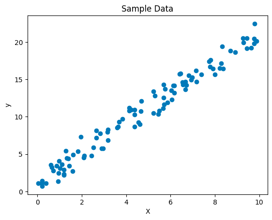

This scatter plot should show a general upward trend, indicating a positive correlation between X and y.

Data Split : Training and Testing Sets

Next, we’ll split our data into training and testing sets:

X_train, X_test, y_train, y_test = train_test_split(df[['X']], df['y'], test_size=0.2, random_state=42)

Training the Model

Now, let’s create and train our linear regression model:

model = LinearRegression()
model.fit(X_train, y_train)

With our model trained, we can make predictions on the test set:

y_pred = model.predict(X_test)

Model Performance

To evaluate our model’s performance, we’ll calculate the Mean Squared Error (MSE) and R-squared (R²) score:

mse = mean_squared_error(y_test, y_pred)
r2 = r2_score(y_test, y_pred)

print(f"Mean Squared Error: {mse:.4f}")
print(f"R-squared Score: {r2:.4f}")

##Output
#Mean Squared Error: 0.9178
#R-squared Score: 0.9577

These metrics give us an idea of how well our model is performing. A lower MSE indicates better predictions, while an R² closer to 1 suggests a better fit.

Model Prediction

Finally, let’s visualize our model’s predictions alongside the original data:

plt.scatter(df['X'], df['y'], color='blue', label='Data')
plt.plot(X_test, y_pred, color='red', label='Predictions')
plt.xlabel('X')
plt.ylabel('y')
plt.title('Linear Regression Model')
plt.legend()
plt.show()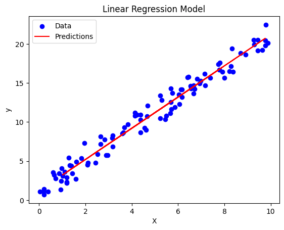

This plot should show our original data points and the line of best fit determined by our linear regression model.

Interpreting the Results

After running this code, you’ll have a trained linear regression model. The model’s coefficients (slope and intercept) can be accessed using:

print(f"Slope: {model.coef_[0]:.4f}")
print(f"Intercept: {model.intercept_:.4f}")

##Output
#Slope: 1.9981
#Intercept: 1.2063

These values tell us how X relates to y in our model. The slope indicates how much y changes for a unit increase in X, while the intercept represents the predicted y value when X is 0.

Real-World Applications

Linear regression finds applications in various fields:

1. Economics: Predicting economic indicators based on various factors.
2. Finance: Analyzing stock prices and portfolio performance.
3. Marketing: Understanding the relationship between advertising spend and sales.
4. Healthcare: Predicting patient outcomes based on treatment variables.
5. Environmental Science: Modeling climate patterns and their effects.

Conclusion

Linear regression is a powerful tool in the machine learning toolkit. Its simplicity, interpretability, and wide range of applications make it an essential technique to master. By understanding its principles and implementing it in Python, you’re well on your way to tackling more complex machine learning challenges.

Remember, while linear regression is a great starting point, it’s often just the beginning. As you grow in your machine learning journey, you’ll discover when to use linear regression and when to explore more advanced techniques.

FAQs:

Q1. What’s the difference between simple linear regression and multiple linear regression?

Simple linear regression involves only one independent variable, while multiple linear regression uses two or more independent variables to predict the dependent variable.

Q2. How do I know if linear regression is appropriate for my data?

Check if there’s a linear relationship between variables, ensure your data meets the assumptions (linearity, independence, homoscedasticity, normality), and consider the nature of your problem. If these conditions are met, linear regression could be appropriate.

Q3. What does the R-squared value tell me about my model?

R-squared represents the proportion of variance in the dependent variable that’s predictable from the independent variable(s). It ranges from 0 to 1, with 1 indicating perfect prediction and 0 indicating the model doesn’t explain any variability in the data.

Q4. Can linear regression be used for classification problems?

While linear regression is primarily used for continuous outcomes, a variant called logistic regression is used for binary classification problems. For multi-class classification, other techniques are typically more appropriate.

Q5. How can I improve my linear regression model if it’s not performing well?

You can try adding more relevant features, removing outliers, transforming variables, using polynomial terms for non-linear relationships, or considering regularization techniques to prevent overfitting.

Q6. Is it possible to have too many variables in a linear regression model?

Yes, having too many variables can lead to overfitting, especially if you have a small dataset. This is known as the “curse of dimensionality.” Feature selection techniques or regularization can help address this issue.

Learn more about machine learning and other topics

• Machine Learning: A Quick Refresher & Ultimate Cheat Sheet
• Machine Learning Algorithms: How To Evaluate The Pros & Cons
• The Ultimate Cheat Sheet for Deep Learning
• Cloud Load Balancing: How To Choose?
• AWS Redshift Vs Snowflake: How To Choose?
• NoSQL Vs SQL Databases: An Ultimate Guide To Choose